Get Started

Algorithm outline

The parametric g-formula estimator of the noniterative conditional expectation (NICE) requires the specification of models for the joint density of the confounders, treatments, and outcomes over time. The algorithm has three steps: (1) Parametric estimation, (2) Monte Carlo simulation , and (3) Calculation of risk/mean under each intervention.

Parametric estimation: (a) estimate the conditional densities of each covariate given past covariate history by fitting user-specified regression models, (b) estimate the discrete hazard (for survival outcome) or mean (for binary/continuous end of follow-up) of the outcome conditional on past covariate history by fitting a user-specified regression model, (c) if the event of interest is subject to competing events and competing events are not treated as censoring events, estimate the conditional probability of the competing event conditional on past covariate history by fitting user-specified regression model for the competing event.
Monte Carlo simulation: (a) generate a new dataset which is usually larger than original dataset, for each covariate, generate simulated values at each time step using the estimated covariate models from step (1), (b) for the covariates that are to undergo intervention, their values are assigned according to the user-specified intervention rule, (c) obtain the discrete hazard / mean of the outcome based on the estimated outcome model from step (1), (d) if the event of interest is subject to competing events and competing events are not treated as censoring events, obtain the discrete hazard of the competing event based on the estimated competing model from step (1).
Calculation of risk/mean under each intervention: for binary/continuous end of follow-up, the final estimate is the mean of the estimated outcome of all individuals in the new dataset computed from Step (2). For survival outcome, the final estimate is obtained by calculating the mean of cumulative risks for all individuals using the discrete hazards computed from step (2).

Arguments:

ParametricGformula(obs_data, id, time_name, ...)

G-formula estimation under parametric models.

class pygformula.parametric_gformula.ParametricGformula(obs_data, id, time_name, outcome_name, ymodel, covnames=None, covtypes=None, covmodels=None, int_descript=None, custom_histvars=None, custom_histories=None, covfits_custom=None, covpredict_custom=None, ymodel_fit_custom=None, ymodel_predict_custom=None, nsamples=0, compevent_name=None, compevent_model=None, compevent_cens=False, intcomp=None, censor_name=None, censor_model=None, model_fits=False, boot_diag=False, ipw_cutoff_quantile=None, ipw_cutoff_value=None, outcome_type=None, trunc_params=None, time_thresholds=None, time_points=None, n_simul=None, sim_trunc=True, baselags=False, visitprocess=None, restrictions=None, yrestrictions=None, compevent_restrictions=None, basecovs=None, parallel=False, ncores=None, ref_int=None, ci_method=None, seed=None, save_path=None, save_results=False, **interventions)

G-formula estimation under parametric models.

Parameters:

obs_data (DataFrame) – A data frame containing the observed data.
id (Str) – A string specifying the name of the id variable in obs_data.
time_name (Str) – A string specifying the name of the time variable in obs_data.
outcome_name (Str) – A string specifying the name of the outcome variable in obs_data.
ymodel (Str) – A string specifying the model statement for the outcome variable.
covnames (List, default is None) – A list of strings specifying the names of the time-varying covariates in obs_data.
covtypes (List, default is None) – A list of strings specifying the “type” of each time-varying covariate included in covnames. The supported types: “binary”, “normal”, “categorical”, “bounded normal”, “zero-inflated normal”, “truncated normal”, “absorbing”, “categorical time”, “square time” and “custom”. The list must be the same length as covnames and in the same order.
covmodels (List, default is None) – A list of strings, where each string is the model statement of the time-varying covariate. The list must be the same length as covnames and in the same order. If a model is not required for a certain covariate, it should be set to ‘NA’ at that index.
int_descript (List, default is None) – A list of strings, each of which describes a user-specified intervention.
custom_histvars (List, default is None) – A list of strings, each of which specifies the names of the time-varying covariates with user-specified custom histories.
custom_histories (List, default is None) – A list of functions, each function is the user-specified custom history functions for covariates. The list should be the same length as custom_histvars and in the same order.
covfits_custom (List, default is None) – A list, each element could be ‘NA’ or a user-specified fit function. The non-NA value is set for the covariates with custom type. The ‘NA’ value is set for other covariates. The list must be the same length as covnames and in the same order.
covpredict_custom (List, default is None) – A list, each element could be ‘NA’ or a user-specified predict function. The non-NA value is set for the covariates with custom type. The ‘NA’ value is set for other covariates. The list must be the same length as covnames and in the same order.
ymodel_fit_custom (Function, default is None) – A user-specified fit function for the outcome variable.
ymodel_predict_custom (Function, default is None) – A user-specified predict function for the outcome variable.
nsamples (Int, default is 0) – An integer specifying the number of bootstrap samples to generate.
compevent_name (Str, default is None) – A string specifying the name of the competing event variable in obs_data. Only applicable for survival outcomes.
compevent_model (Str, default is None) – A string specifying the model statement for the competing event variable. Only applicable for survival outcomes.
compevent_cens (Bool, default is False) – A boolean value indicating whether to treat competing events as censoring events.
intcomp (List, default is None) – List of two numbers indicating a pair of interventions to be compared by a hazard ratio.
censor_name (Str, default is None) – A string specifying the name of the censoring variable in obs_data. Only applicable when using inverse probability weights to estimate the natural course means / risk from the observed data.
censor_model (Str, default is None) – A string specifying the model statement for the censoring variable. Only applicable when using inverse probability weights to estimate the natural course means / risk from the observed data.
model_fits (Bool, default is False) – A boolean value indicating whether to return the parameter estimates of the models.
boot_diag (Bool, default is False) – A boolean value indicating whether to return the parametric g-formula estimates as well as the coefficients, standard errors, and variance-covariance matrices of the parameters of the fitted models in the bootstrap samples.
ipw_cutoff_quantile (Float, default is None) – Percentile value for truncation of the inverse probability weights.
ipw_cutoff_value (Float, default is None) – Absolute value for truncation of the inverse probability weights.
outcome_type (Str, default is None) – A string specifying the “type” of outcome. The possible “types” are: “survival”, “continuous_eof”, and “binary_eof”.
trunc_params (List, default is None) – A list, each element could be ‘NA’ or a two-element list. If not ‘NA’, the first element specifies the truncated value and the second element specifies the truncated direction (‘left’ or ‘right’). The non-NA value is set for the truncated normal covariates. The ‘NA’ value is set for other covariates. The list should be the same length as covnames and in the same order.
time_thresholds (List, default is None) – A list of integers that splits the time points into different intervals. It is used to create the variable “categorical time”.
time_points (Int, default is K+1) – An integer indicating the number of time points to simulate. It is set equal to the maximum number of records (K) that obs_data contains for any individual plus 1, if not specified by users.
n_simul (Int, default is M) – An integer indicating the number of subjects for whom to simulate data. It is set equal to the number (M) of subjects in obs_data, if not specified by users.
sim_trunc (Bool, default is True) – A boolean value indicating if the simulated values of normal covariates are truncated by the observed ranges.
baselags (Bool, default is False) – A boolean value specifying the convention used for lagi and lag_cumavgi terms in the model statements when pre-baseline times are not included in obs_data and when the current time index, t, is such that t < i. If this argument is set to False, the value of all lagi and lag_cumavgi terms in this context are set to 0 (for non-categorical covariates) or the reference level (for categorical covariates). If this argument is set to True, the value of lagi and lag_cumavgi terms are set to their values at time 0. The default is False.
visitprocess (List, default is None) – List of lists. Each inner list contains its first entry the covariate name of a visit process; its second entry the name of a covariate whose modeling depends on the visit process; and its third entry the maximum number of consecutive visits that can be missed before an individual is censored.
restrictions (List, default is None) – List of lists. Each inner list contains its first entry the covariate name of that its deterministic knowledge is known; its second entry is a dictionary whose key is the conditions which should be True when the covariate is modeled, the third entry is the value that is set to the covariate during simulation when the conditions in the second entry are not True.
yrestrictions (List, default is None) – List of lists. For each inner list, its first entry is a dictionary whose key is the conditions which should be True when the outcome is modeled, the second entry is the value that is set to the outcome during simulation when the conditions in the first entry are not True.
compevent_restrictions (List, default is None) – List of lists. For each inner list, its first entry is a dictionary whose key is the conditions which should be True when the competing event is modeled, the second entry is the value that is set to the competing event during simulation when the conditions in the first entry are not True. Only applicable for survival outcomes.
basecovs (List, default is None) – A list of strings specifying the names of baseline covariates in obs_data. These covariates should not be included in covnames.
parallel (Bool, default is False) – A boolean value indicating whether to parallelize simulations of different interventions to multiple cores.
ncores (Int, default is 1) – An integer indicating the number of cores used in parallelization. It is set to 1 if not specified by users.
ref_int (Int, default is 0) – An integer indicating the intervention to be used as the reference for calculating the end-of-follow-up mean/risk ratio and mean/risk difference. 0 denotes the natural course, while subsequent integers denote user-specified interventions in the order that they are named in interventions. It is set to 0 if not specified by users.
ci_method (Str, default is "percentile") – A string specifying the method for calculating the bootstrap 95% confidence intervals, if applicable. The options are “percentile” and “normal”. It is set to “percentile” if not specified by users.
seed (Int, default is 1234) – An integer indicating the starting seed for simulations and bootstrapping. It is set to 1234 if not specified by users.
save_path (Path, default is None) – A path to save all the returned results. A folder will be created automatically in the current working directory if the save_path is not specified by users.
save_results (Bool, default is False) – A boolean value indicating whether to save all the returned results to the save_path.
**interventions (Dict, default is None) – A dictionary whose key is the treatment name in the intervention with the format Intervention{id}_{treatment_name}, value is a list that contains the intervention function, values required by the function, and a list of time points in which the intervention is applied.

Example

The observational dataset example_data_basicdata_nocomp consists of 13,170 observations on 2,500 individuals with a maximum of 7 follow-up times. The dataset contains the following variables:

id: Unique identifier for each individual.

t0: Time index.

L1: Binary time-varying covariate.

L2: Continuous time-varying covariate.

L3: Categorical baseline covariate.

A: Binary treatment variable.

Y: Outcome of interest; time-varying indicator of failure.

We are interested in the risk by the end of follow-up under the static interventions ‘‘Never treat’’ (set treatment to 0 at all times) and ‘‘Always treat’’ (set treatment to 1 at all times).

First, import the g-formula method ParametricGformula:
```
from pygformula import ParametricGformula
```
Then, load the data (here is an example of loading simulated data in the package, users can also load their own data) as required pandas DataFrame type
```
from pygformula.data import load_basicdata_nocomp
obs_data = load_basicdata_nocomp()
```
Specify the name of the time variable, and the name of the individual identifier in the input data
```
time_name = 't0'
id = 'id'
```

Specify covariate names, covariate types, and corresponding model statements

covnames = ['L1', 'L2', 'A']
covtypes = ['binary', 'bounded normal', 'binary']
covmodels = ['L1 ~ lag1_A + lag2_A + lag_cumavg1_L1 + lag_cumavg1_L2 + L3 + t0',
             'L2 ~ lag1_A + L1 + lag_cumavg1_L1 + lag_cumavg1_L2 + L3 + t0',
             'A ~ lag1_A + L1 + L2 + lag_cumavg1_L1 + lag_cumavg1_L2 + L3 + t0']

If there are baseline covariates (i.e., covariate with same value at all times) in the model statement, specify them in the ‘‘basecovs’’ argument:

basecovs = ['L3']

Specify the static interventions of interest:

from pygformula.interventions import static

time_points = np.max(np.unique(obs_data[time_name])) + 1
int_descript = ['Never treat', 'Always treat']

Intervention1_A = [static, np.zeros(time_points)],
Intervention2_A = [static, np.ones(time_points)],

Specify the outcome name, outcome model statement, and the outcome type

outcome_name = 'Y'
ymodel = 'Y ~ L1 + L2 + L3 + A + lag1_A + lag1_L1 + lag1_L2 + t0'
outcome_type = 'survival'

Speficy all the arguments in the “ParametricGformula” class and call its “fit” function:

g = ParametricGformula(obs_data = obs_data, id = id, time_name=time_name,
    covnames=covnames, covtypes=covtypes,
    covmodels=covmodels, basecovs=basecovs,
    time_points=time_points,
    Intervention1_A = [static, np.zeros(time_points)],
    Intervention2_A = [static, np.ones(time_points)],
    outcome_name=outcome_name, ymodel=ymodel,
    outcome_type = outcome_type)

g.fit()

Finally, get the output:
- “Intervention”: the name of natural course intervention and user-specified interventions.
- “NP-risk”: the nonparametric estimates of the natural course risk.
- “g-formula risk”: the parametric g-formula estimates of each interventions.
- “Risk Ratio (RR)”: the risk ratio comparing each intervention and reference intervention.
- “Risk Difference (RD)”: the risk difference comparing each intervention and reference intervention.

In the output table, the g-formula risk results under the specified interventions are shown, as well as the natural course. Furthermore, the nonparametric risk under the natural course is provided, which can be used to assess model misspecification of parametric g-formula. The risk ratio and risk difference comparing the specific intervention and the reference intervention (set to natural course by default) are also calculated.

Users can also get the standard errors and 95% confidence intervals of the g-formula estimates by specifying the ‘‘nsamples’’ argument. For example, specifying ‘‘nsamples’’ as 20 with parallel processing using 8 cores:

g = ParametricGformula(obs_data = obs_data, id = id, time_name=time_name,
    time_points = time_points,
    Intervention1_A = [static, np.zeros(time_points)],
    Intervention2_A = [static, np.ones(time_points)],
    covnames=covnames, covtypes=covtypes,
    covmodels=covmodels, basecovs=basecovs,
    outcome_name=outcome_name, ymodel=ymodel, outcome_type=outcome_type,
    nsamples=20, parallel=True, ncores=8)
g.fit()

The package will return following results:

The result table contains 95% lower bound and upper bound for the risk, risk difference and risk ratio for all interventions.

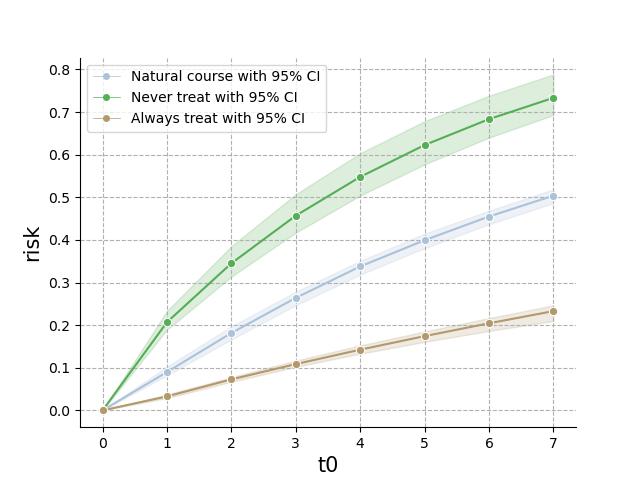
The pygformula also provides plots for risk curves of interventions, which can be called by:

g.plot_interventions()

It will return the g-formula risk (with 95% confidence intervals if using bootstrap samples) at all follow-up times under each intervention:

User can also get the plots of parametric and nonparametric estimates of the risks and covariate means under natural course by:

g.plot_natural_course()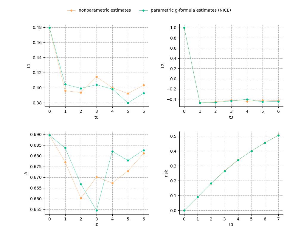

Running example [code]:

import numpy as np
from pygformula import ParametricGformula
from pygformula.interventions import static
from pygformula.data import load_basicdata_nocomp

obs_data = load_basicdata_nocomp()
time_name = 't0'
id = 'id'

covnames = ['L1', 'L2', 'A']
covtypes = ['binary', 'bounded normal', 'binary']
covmodels = ['L1 ~ lag1_A + lag2_A + lag_cumavg1_L1 + lag_cumavg1_L2 + L3 + t0',
           'L2 ~ lag1_A + L1 + lag_cumavg1_L1 + lag_cumavg1_L2 + L3 + t0',
           'A ~ lag1_A + L1 + L2 + lag_cumavg1_L1 + lag_cumavg1_L2 + L3 + t0']

basecovs = ['L3']

outcome_name = 'Y'
ymodel = 'Y ~ L1 + L2 + L3 + A + lag1_A + lag1_L1 + lag1_L2 + t0'
outcome_type = 'survival'

time_points = np.max(np.unique(obs_data[time_name])) + 1
int_descript = ['Never treat', 'Always treat']

g = ParametricGformula(obs_data = obs_data, id = id, time_name=time_name,
             time_points = time_points, int_descript = int_descript,
             covnames=covnames, covtypes=covtypes,
             covmodels=covmodels, basecovs=basecovs,
             outcome_name=outcome_name, ymodel=ymodel, outcome_type=outcome_type,
             Intervention1_A = [static, np.zeros(time_points)],
             Intervention2_A = [static, np.ones(time_points)],
             nsamples=20, parallel=True, ncores=8)
g.fit()
g.plot_natural_course()
g.plot_interventions()