Covariate models
To model the joint densities of covariates in g-formula, the conditional densities of each covariate given past covariate history are estimated. Users can specify the covariate histories by the pre-coded functions of histories or custom histories. The package provides options of modeling different covariate distributions , which contains ‘‘binary’’, ‘‘normal’’, ‘‘categorical’’, ‘‘bounded normal’’, ‘‘zero-inflated normal’’, ‘‘truncated normal’’, ‘‘absorbing’’, ‘‘categorical time’’ and ‘‘square time’’. Once the covariate model and covariate distribution are specified, the pygformula will fit a pooled (over time) parametric model for each covariate. The custom covariate type is also allowed if users have their own covariate distribution, which should be set to “custom” in corresponding covariate types.
Functions of covariate histories
Pre-coded histories
The package provides three pre-coded functions (‘‘lag’’, ‘‘cumavg’’, ‘‘lag_cumavg’’) for users to specify the covariate histories.
‘‘lag’’: For any covariate L, specifying lagi_L will add a variable to the input dataset, which contains the i-th lag of L relative to the current follow-up time k. For example, lag1_L means the value of L at the time k-1, lag2_L means the value of L at the time k-2 etc. The value is set to 0 if k < i if there is no pre-baseline times.
‘‘cumavg’’: For any covariate L, specifying cumavg_L will add a variable to the input dataset, which contains the cumulative average of L up until the current follow-up time k.
‘‘lag_cumavg’’: For any covariate L, specifying lag_cumavgi_L will add a variable to the input dataset, which contains the i-th lag of the cumulative average of L relative to the current follow-up time k. The value is set to 0 if k < i if there is no pre-baseline times.
An example for specifying the covariate model for covariate L1 based on the history functions:
L1 ~ lag1_L1 + cumavg_L1 + lag_cumavg1_L1 + L3 + t0
Note: for more covariate transformations (e.g., polynomial terms, spline terms), see patsy for specification.
Custom histories
If users wish to use history functions that are not in the three pre-coded history functions, the package provides ‘‘custom_histvars’’ and ‘‘custom_histories’’ for users to specify their own history functions for corresponding covariates.
Arguments |
Description |
|---|---|
custom_histvars |
(Optional) A list of strings, each of which specifies the names of the time-varying covariates with user-specified custom histories. |
custom_histories |
(Optional) A list of functions, each function is the user-specified custom history functions for covariates. The list should be the same length as custom_histvars and in the same order. |
For each custom history function, the input should be the parameters (not necessary to use all):
pool: A DataFrame that contains the observed or simulated data up to time t.
histvar: A string that specifies the name of the variable for which this history function is to be applied.
time_name: A string specifying the name of the time variable in pool.
t: An integer specifying the current time index.
id: A string specifying the name of the ID variable in the pool.
The function output is a dataframe ‘‘pool’’ with the new column of the historical term created.
The following is an example of creating historical functions for covariates ‘’L1’’, ‘’L2’’ and ‘’A’’ by the function ‘ave_last3’. This function generates the average of the three most recent values of the covariate (when the t=0, it takes the current value at time 0; when t=1, it takes the average of the covariate values at times 0 and 1). The new historical covariates are named as ave_last3_L1, ave_last3_L2, and ave_last3_A.
Sample syntax:
def ave_last3(pool, histvar, time_name, t, id):

  def avg_func(df, time_name, t, histvar):
      if t < 3:
          avg_values = np.mean((df[(df[time_name] >= 0) & (df[time_name] <= t)][histvar]))
      else:
          avg_values = np.mean((df[(df[time_name] > t - 3) & (df[time_name] <= t)][histvar]))
      return avg_values

  valid_pool = pool.groupby(id_name).filter(lambda x: max(x[time_name]) >= t)
  pool.loc[pool[time_name] == t, '_'.join(['ave_last3', str(histvar)])] = list(valid_pool.groupby(id_name).apply(
      avg_func, time_name=time_name, t=t, histvar=histvar))

return pool

custom_histvars = ['L1', 'L2', 'A']
custom_histories = [ave_last3, ave_last3, ave_last3]

g = ParametricGformula(..., custom_histvars = custom_histvars, custom_histories=custom_histories, ...)
The ave_last3 function has been included in the package, users can also call this function by:
from pygformula.parametric_gformula.histories import ave_last3
Different covariate distributions
To specify a parametric model for each covariate in pygformula, users need to specify the following arguments:
Arguments |
Description |
|---|---|
covnames |
(Required) A list of strings specifying the names of the time-varying covariates in obs_data. |
covtypes |
(Required) A list of strings specifying the “type” of each time-varying covariate included in covnames. The supported types: “binary”, “normal”, “categorical”, “bounded normal”, “zero-inflated normal”, “truncated normal”, “absorbing”, “categorical time”, “square time” and “custom”. The list must be the same length as covnames and in the same order. |
covmodels |
(Required) A list of strings, where each string is the model statement of the time-varying covariate. The list must be the same length as covnames and in the same order. If a model is not required for a certain covariate, it should be set to ‘NA’ at that index. |
basecovs |
(Optional) A list of strings specifying the names of baseline covariates in obs_data. These covariates should not be included in covnames. |
trunc_params |
(Optional) A list, each element could be ‘NA’ or a two-element list. If not ‘NA’, the first element specifies the truncated value and the second element specifies the truncated direction (‘left’ or ‘right’). The non-NA value is set for the truncated normal covariates. The ‘NA’ value is set for other covariates. The list should be the same length as covnames and in the same order. |
time_thresholds |
(Optional) A list of integers that splits the time points into different intervals. It is used to create the variable “categorical time”. |
Users need to specify the names of time-varying covariates in ‘‘covnames’’, the distribution type of each covariate in ‘‘covtypes’’, as well as the model statement for each covariate in ‘‘covmodels’’. In addition, if there are time-fixed baseline covariates, they should be specified in the argument ‘‘basecovs’’. If the covariate type is ‘‘truncated normal’’, the ‘‘trunc_params’’ argument should be also specified which contains the required truncated direction and truncated value. If the covariate type is ‘‘categorical time’’, users should also define the ‘‘time_thresholds’’ argument to create a desired categorization of time. In the following, this section shows examples for different covariate distributions to show how to specify the above arguments in specific examples.
Note
For the ‘‘covmodels’’ argument which specifies the model statement for each covariate, users need to be careful to avoid the loop between covariates, i.e., in each covariate model statement, the independent variable and dependent variable should follow the direction in the DAG (directed acyclic graph). For example, if the covariate A is the dependent variable of the covariate B (A ~ B), then the covariate B should not be the dependent variable of the covariate A (B ~ A).
Binary
When the covariate is binary, in the fitting step, the input data is used to estimate a generalized linear model where the family function is binomial. Then, in the simulation step, the mean of the covariate conditional on history at each time step is estimated via the coefficients of the fitted model, the covariate values are simulated by sampling from a Bernoulli distribution with parameter the conditional probability.
Sample syntax:
An example where the covariate ‘’L1’’ is binomial distribution
covnames = [ 'L1', 'A']
covtypes = ['binary', 'binary']
covmodels = ['L1 ~ lag1_A + lag2_A + lag_cumavg1_L1 + lag_cumavg1_L2 + L3 + t0',
             'A ~ lag1_A + L1 + L2 + lag_cumavg1_L1 + lag_cumavg1_L2 + L3 + t0']

basecovs = ['L3']

g = ParametricGformula(..., covnames = covnames, covtypes = covtypes, covmodels = covmodels, basecovs = basecovs, ...)
Running example [code]:
import numpy as np
from pygformula import ParametricGformula
from pygformula.interventions import static
from pygformula.data import load_basicdata_nocomp

obs_data = load_basicdata_nocomp()
time_name = 't0'
id = 'id'

covnames = ['L1', 'A']
covtypes = ['binary', 'binary']
covmodels = ['L1 ~ lag1_A + lag2_A + lag_cumavg1_L1 + L3 + t0',
           'A ~ lag1_A + L1 + lag_cumavg1_L1 + L3 + t0']

basecovs = ['L3']

outcome_name = 'Y'
ymodel = 'Y ~ L1 + A + lag1_A + lag1_L1 + L3 + t0'
outcome_type = 'survival'

time_points = np.max(np.unique(obs_data[time_name])) + 1
int_descript = ['Never treat', 'Always treat']

g = ParametricGformula(obs_data = obs_data, id = id, time_name=time_name,
             time_points = time_points, int_descript = int_descript,
             Intervention1_A = [static, np.zeros(time_points)],
             Intervention2_A = [static, np.ones(time_points)],
             covnames=covnames, covtypes=covtypes,
             covmodels=covmodels, basecovs=basecovs,
             outcome_name=outcome_name, ymodel=ymodel, outcome_type=outcome_type)
g.fit()
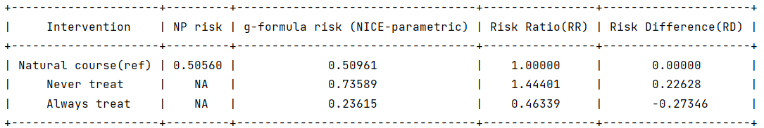
Output:

Note that in this section, all demonstration examples use the same static interventions (‘‘Never treat’’ and ‘‘Always treat’’), and are applied in the survival outcome case. Please refer to Interventions for more types of interventions, and Outcome model for more types of outcomes.
Normal
When the covariate is normal, in the fitting step, the input data is used to estimate a generalized linear model where the family function is gaussian. Then, in the simulation step, the mean of the covariate conditional on history at each time step is estimated via the coefficients of the fitted model, the covariate values are simulated by sampling from a normal distribution with mean this conditional mean and variance the residual mean squared error from the fitted model. Values generated outside the observed range for the covariate are set to the minimum or maximum of this range.
Sample syntax:
covnames = ['L2', 'A']
covtypes = ['normal', 'binary']
covmodels = ['L2 ~ lag1_A + lag_cumavg1_L2 + L3 + t0',
             'A ~ lag1_A + L2 + lag_cumavg1_L2 + L3 + t0']

basecovs = ['L3']

g = ParametricGformula(..., covnames = covnames, covtypes = covtypes, covmodels = covmodels, basecovs = basecovs, ...)
Running example [code]:
import numpy as np
from pygformula import ParametricGformula
from pygformula.interventions import static
from pygformula.data import load_basicdata_nocomp

obs_data = load_basicdata_nocomp()
time_name = 't0'
id = 'id'

covnames = ['L2', 'A']
covtypes = ['normal', 'binary']
covmodels = ['L2 ~ lag1_A + lag_cumavg1_L2 + L3 + t0',
           'A ~ lag1_A + L2 + lag_cumavg1_L2 + L3 + t0']

basecovs = ['L3']

outcome_name = 'Y'
ymodel = 'Y ~ L2 + A + lag1_A + L3 + t0'
outcome_type = 'survival'

time_points = np.max(np.unique(obs_data[time_name])) + 1
int_descript = ['Never treat', 'Always treat']

g = ParametricGformula(obs_data = obs_data, id = id, time_name=time_name,
          time_points = time_points, int_descript = int_descript,
          Intervention1_A = [static, np.zeros(time_points)],
          Intervention2_A = [static, np.ones(time_points)],
          covnames=covnames, covtypes=covtypes,
          covmodels=covmodels, basecovs=basecovs,
          outcome_name=outcome_name, ymodel=ymodel, outcome_type=outcome_type)
g.fit()
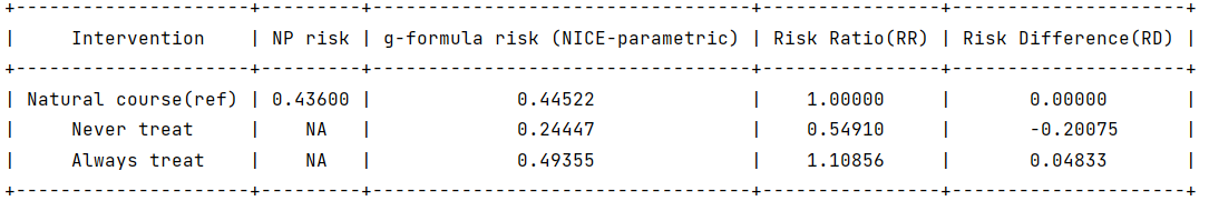
Output:

Categorical
When the covariate is categorical, in the fitting step, the input data is used to estimate a multinomial logistic regression model. Then, in the simulation step, the probability that a covariate takes a particular level conditional on history is estimated via the coefficients of the fitted model. The covariate values are simulated at each time step by sampling from a multinoulli distribution with parameters these estimated conditional probabilities of the fitted model.
Sample syntax:
covnames = [ 'L', 'A']
covtypes = ['categorical', 'binary']
covmodels = [ 'L ~ C(lag1_L) + t0',
              'A ~ C(L) + C(lag1_L) + t0']

g = ParametricGformula(..., covnames = covnames, covtypes = covtypes, covmodels = covmodels,...)
Note that when the covariate model statement contains any categorical variable, such as ‘‘lag1_L’’ or ‘‘L’’, e.g., in the example above, users need to add a ‘‘C( )’’ on the variable indicating it’s categorical.
Running example [code]:
import numpy as np
from pygformula import ParametricGformula
from pygformula.interventions import static
from pygformula.data import load_categorical

obs_data = load_categorical()
time_name = 't0'
id = 'id'

covnames = [ 'L', 'A']
covtypes = ['categorical', 'binary']
covmodels = [ 'L ~ C(lag1_L) + t0',
              'A ~ C(L) + C(lag1_L) + t0']

outcome_name = 'Y'
ymodel = 'Y ~ C(lag1_L) + A'

time_points = np.max(np.unique(obs_data[time_name])) + 1
int_descript = ['Never treat', 'Always treat']

g = ParametricGformula(obs_data = obs_data, id = id, time_name=time_name,
           time_points = time_points,int_descript = int_descript,
           Intervention1_A = [static, np.zeros(time_points)],
           Intervention2_A = [static, np.ones(time_points)],
           covnames=covnames,  covtypes=covtypes,
           covmodels=covmodels, outcome_name=outcome_name,
           ymodel=ymodel, outcome_type='survival')
g.fit()
Output:

Bounded normal
When the covariate is bounded normal, the observed covariate values are first standardized to the interval [0, 1], inclusive, by subtracting the minimum value and dividing by the range. In the fitting step, the input data with standardized covariate is used to estimate a generalized linear model where the family function is gaussian. In the simulation step, the mean of the covariate conditional on history at each time step is estimated via the coefficients of the fitted model, the standardized covariate values are simulated by sampling from a normal distribution with mean this conditional mean and variance the residual mean squared error from the fitted model. Finally, the simulated standardized values are then transformed back to the original scale, and values generated outside the observed range for the covariate are set to the minimum or maximum of this range.
Sample syntax:
covnames = ['L2', 'A']
covtypes = ['bounded normal', 'binary']
covmodels = ['L2 ~ lag1_A + lag_cumavg1_L2 + L3 + t0',
             'A ~ lag1_A + L2 + lag_cumavg1_L2 + L3 + t0']

basecovs = ['L3']

g = ParametricGformula(..., covnames = covnames, covtypes = covtypes, covmodels = covmodels, basecovs = basecovs, ...)
Running example [code]:
import numpy as np
from pygformula import ParametricGformula
from pygformula.interventions import static
from pygformula.data import load_basicdata_nocomp

obs_data = load_basicdata_nocomp()
time_name = 't0'
id = 'id'

covnames = ['L2', 'A']
covtypes = ['bounded normal', 'binary']
covmodels = ['L2 ~ lag1_A + lag_cumavg1_L2 + L3 + t0',
           'A ~ lag1_A + L2 + lag_cumavg1_L2 + L3 + t0']

basecovs = ['L3']

outcome_name = 'Y'
ymodel = 'Y ~ L2 + A + lag1_A + L3 + t0'
outcome_type = 'survival'

time_points = np.max(np.unique(obs_data[time_name])) + 1
int_descript = ['Never treat', 'Always treat']

g = ParametricGformula(obs_data = obs_data, id = id, time_name=time_name,
         time_points = time_points, int_descript = int_descript, intcomp=[1, 2],
         Intervention1_A = [static, np.zeros(time_points)],
         Intervention2_A = [static, np.ones(time_points)],
         covnames=covnames, covtypes=covtypes,
         covmodels=covmodels, basecovs=basecovs,
         outcome_name=outcome_name, ymodel=ymodel, outcome_type=outcome_type)
g.fit()
Output:

Zero-inflated normal
When the covariate is zero-inflated normal, in the fitting step, the input data will be added an indicator variable by setting the covariate values that are greater than 0 to 1 and keeping the original zeros values. The input data with the added indicator variable is used to first fit a generalized linear model where the family function is binomial. Then, the input data with positive values at the covariate is used to fit a generalized linear model where the family function is gaussian. In the simulation step, the simulated covariate values are created by first generating an indicator of whether the covariate value is zero or non-zero from a Bernoulli distribution with the parameter the probability from the first fitted model. Covariate values are then generated from a normal distribution with the mean of the second fitted model and multiplied by the generated zero indicator. The simulated non-zero covariate values that fall outside the observed range are set to the minimum or maximum of the range of non-zero observed values of the covariate.
Sample syntax:
covnames = ['L', 'A']
covtypes = ['zero-inflated normal', 'binary']
covmodels = ['L ~ lag1_L + lag1_A + t0',
              'A ~ lag1_A + L + t0']

g = ParametricGformula(..., covnames = covnames, covtypes = covtypes, covmodels = covmodels, ...)
Running example [code]:
import numpy as np
from pygformula import ParametricGformula
from pygformula.interventions import static
from pygformula.data import load_zero_inflated_normal

obs_data = load_zero_inflated_normal()
time_name = 't0'
id = 'id'

covnames = ['L', 'A']
covtypes = ['zero-inflated normal', 'binary']
covmodels = ['L ~ lag1_L + lag1_A + t0',
              'A ~ lag1_A + L + t0']

outcome_name = 'Y'
ymodel = 'Y ~ L + A + t0'
outcome_type = 'survival'

time_points = np.max(np.unique(obs_data[time_name])) + 1
int_descript = ['Never treat', 'Always treat']

g = ParametricGformula(obs_data = obs_data, id = id, time_name=time_name,
             time_points = time_points, int_descript = int_descript,
             Intervention1_A = [static, np.zeros(time_points)],
             Intervention2_A = [static, np.ones(time_points)],
             covnames=covnames, covtypes=covtypes, covmodels=covmodels,
             outcome_name=outcome_name, ymodel=ymodel, outcome_type=outcome_type)
g.fit()
Output:

Truncated normal
When the covariate is truncated normal, in the fitting step, the input data is used to fit a truncated normal regression model. In the simulation step, the mean of the covariate conditional on history at each time step is estimated via the coefficients of the fitted model, then the simulated covariate values are generated by sampling from a truncated normal distribution with the covariate mean from the fitted model. The generated covariate values that fall outside the observed range are set to the minimum or maximum of the observed range.
Sample syntax:
covnames = ['L', 'A']
covtypes = ['truncated normal', 'binary']
covmodels = ['L ~ lag1_A + lag1_L + t0',
             'A ~ lag1_A + lag1_L + L + t0']

trunc_params = [[1, 'right'], 'NA']

g = ParametricGformula(..., covnames = covnames, covtypes = covtypes, covmodels = covmodels, trunc_params=trunc_params, ...)
The package supports covariates with one-sided truncation. To specify the covariates, the elements in the ‘‘trunc_params’’ list should follow the same order as ‘‘covnames’’, in the position where its corresponding covariate is truncated normal, it should be a list with two elements, otherwise it should be ‘NA’. In the list of two elements, the first one should be the truncated value of the covariate, and the second one should be the truncated direction (‘left’ or ‘right’) of the covariate.
Running example [code]:
import numpy as np
from pygformula import ParametricGformula
from pygformula.interventions import static
from pygformula.data import load_truncated_normal

obs_data = load_truncated_normal()
time_name = 't0'
id = 'id'

covnames = ['L', 'A']
covtypes = ['truncated normal', 'binary']
covmodels = ['L ~ lag1_A + lag1_L + t0',
           'A ~ lag1_A + lag1_L + L + t0']

trunc_params = [[1, 'right'], 'NA']

outcome_name = 'Y'
ymodel = 'Y ~ L + A + t0'
outcome_type = 'survival'

time_points = np.max(np.unique(obs_data[time_name])) + 1
int_descript = ['Never treat', 'Always treat']

g = ParametricGformula(obs_data = obs_data, id = id, time_name=time_name,
             time_points = time_points, int_descript = int_descript,
             Intervention1_A = [static, np.zeros(time_points)],
             Intervention2_A = [static, np.ones(time_points)],
             covnames=covnames, covtypes=covtypes, covmodels=covmodels,
             trunc_params=trunc_params, outcome_name=outcome_name,
             ymodel=ymodel, outcome_type=outcome_type)
g.fit()
Output:
Absorbing
Absorbing means that once the covariate value switches to 1 at one time step, it stays 1 at all subsequent times. When the covariate is absorbing, the input data records where the value of the covariate at k-1 is 0 for all time steps k is used to fit a generalized linear model where the family function is binomial. Then in the simulation step, the mean of the covariate conditional on history at each time step is estimated via the coefficients of the fitted model, the covariate values are simulated by sampling from a Bernoulli distribution with parameter the conditional mean. Once a 1 is first generated, the covariate value at that time and all subsequent times is set to 1.
Sample syntax:
covnames = ['L', 'A']
covtypes = ['absorbing', 'binary']
covmodels = ['L ~ lag1_L + lag1_A + t0',
             'A ~ lag1_A + L + t0']

g = ParametricGformula(..., covnames = covnames, covtypes = covtypes, covparams = covparams,...)
Running example [code]:
import numpy as np
from pygformula import ParametricGformula
from pygformula.interventions import static
from pygformula.data import load_absorbing_data

obs_data = load_absorbing_data()
time_name = 't0'
id = 'id'

covnames = ['L', 'A']
covtypes = ['absorbing', 'binary']
covmodels = ['L ~ lag1_L + lag1_A + t0',
              'A ~ lag1_A + L + t0']

outcome_name = 'Y'
ymodel = 'Y ~ L + A + t0'
outcome_type = 'survival'

time_points = np.max(np.unique(obs_data[time_name])) + 1
int_descript = ['Never treat', 'Always treat']

g = ParametricGformula(obs_data = obs_data, id = id, time_name=time_name,
             time_points = time_points, int_descript = int_descript,
             covnames=covnames, covtypes=covtypes, covmodels=covmodels,
             Intervention1_A = [static, np.zeros(time_points)],
             Intervention2_A = [static, np.ones(time_points)],
             outcome_name=outcome_name, ymodel=ymodel, outcome_type=outcome_type)
g.fit()
Output:

Time variable
When users assume that the distributions of time-varying covariates depend on a function of the time index, they need to specify an additional time variable. The package has two pre-coded time variable: ‘‘categorical time’’ and ‘‘square time’’. The ‘‘categorical time’’ is a variable that categorizes the time index to different time categories. The ‘‘square time’’ is the squared time index.
Sample syntax of categorical time:
covnames = ['L1', 'L2', 'A', 't0_f']
covtypes = ['binary', 'bounded normal', 'binary', 'categorical time']
covmodels = ['L1 ~ lag1_A + lag2_A + lag_cumavg1_L1 + lag_cumavg1_L2 + L3 + t0 + C(t0_f)',
           'L2 ~ lag1_A + L1 + lag_cumavg1_L1 + lag_cumavg1_L2 + L3 + t0 + C(t0_f)',
           'A ~ lag1_A + L1 + L2 + lag_cumavg1_L1 + lag_cumavg1_L2 + L3 + t0 + C(t0_f)',
           'NA']

time_thresholds = [1, 3, 5]

g = ParametricGformula(..., covnames = covnames, covtypes = covtypes, covmodels = covmodels, time_thresholds = time_thresholds, ...)
The argument ‘‘time_thresholds’’ creates indicators for categorizing the time index, The time index values inside the interval from each adjacent array (right-closed) form a category. for example, setting time_thresholds = [1, 3, 5] in input data with 7 time points means that categorizing the time index to four time categories (category 1: 0 <= time index <=1, category 2 : 1 < time index <=3, category 3 : 3 < time index <=5, category 4 : 5 < time index <= 6).
Users should specify the name of categorical time variable by adding a ‘‘_f’’ after the time name, and specify its type as ‘categorical time’ in covtypes argument. In the covmodels argument, the corresponding position of the categorical time variable should be padded with NA. Note that when using the new categorical time variable in the model statement, e.g., ‘‘t0_f’’ in the syntax example above, C() should be added.
Running example [code]:
import numpy as np
from pygformula import ParametricGformula
from pygformula.interventions import static
from pygformula.data import load_basicdata_nocomp

obs_data = load_basicdata_nocomp()
time_name = 't0'
id = 'id'

covnames = ['L1', 'L2', 'A', 't0_f']
covtypes = ['binary', 'bounded normal', 'binary', 'categorical time']
covmodels = ['L1 ~ lag1_A + lag2_A + lag_cumavg1_L1 + lag_cumavg1_L2 + L3 + t0 + C(t0_f)',
           'L2 ~ lag1_A + L1 + lag_cumavg1_L1 + lag_cumavg1_L2 + L3 + t0 + C(t0_f)',
           'A ~ lag1_A + L1 + L2 + lag_cumavg1_L1 + lag_cumavg1_L2 + L3 + t0 + C(t0_f)',
           'NA']

time_thresholds = [1, 3, 5]

basecovs = ['L3']

outcome_name = 'Y'
ymodel = 'Y ~ L1 + L2 + L3 + A + lag1_A + lag1_L1 + lag1_L2 + t0'
outcome_type = 'survival'

time_points = np.max(np.unique(obs_data[time_name])) + 1
int_descript = ['Never treat', 'Always treat']

g = ParametricGformula(obs_data = obs_data, id = id, time_name=time_name,
    time_points = time_points, time_thresholds = time_thresholds,
    int_descript = int_descript,
    Intervention1_A = [static, np.zeros(time_points)],
    Intervention2_A = [static, np.ones(time_points)],
    covnames=covnames, covtypes=covtypes,
    covmodels=covmodels, basecovs=basecovs,
    outcome_name=outcome_name, ymodel=ymodel, outcome_type=outcome_type)
g.fit()
Output:

Sample syntax of square time:
Note that when the covariate type is ‘‘square time’’, the corresponding covariate name should be set to the merged strings of ‘square’ and the time name in the data, e.g., ‘square_t0’.
covnames = ['L1', 'L2', 'A', 'square_t0']
covtypes = ['binary', 'bounded normal', 'binary', 'square time']
covmodels = ['L1 ~ lag1_A + lag2_A + lag_cumavg1_L1 + lag_cumavg1_L2 + L3 + t0 + square_t0',
           'L2 ~ lag1_A + L1 + lag_cumavg1_L1 + lag_cumavg1_L2 + L3 + t0 + square_t0',
           'A ~ lag1_A + L1 + L2 + lag_cumavg1_L1 + lag_cumavg1_L2 + L3 + t0 + square_t0',
           'NA']

g = ParametricGformula(..., covnames = covnames, covtypes = covtypes, covmodels = covmodels, ...)
Running example [code]:
import numpy as np
from pygformula import ParametricGformula
from pygformula.interventions import static
from pygformula.data import load_basicdata_nocomp

obs_data = load_basicdata_nocomp()
time_name = 't0'
id = 'id'

covnames = ['L1', 'L2', 'A', 'square_t0']
covtypes = ['binary', 'bounded normal', 'binary', 'square time']
covmodels = ['L1 ~ lag1_A + lag2_A + lag_cumavg1_L1 + lag_cumavg1_L2 + L3 + t0 + square_t0',
           'L2 ~ lag1_A + L1 + lag_cumavg1_L1 + lag_cumavg1_L2 + L3 + t0 + square_t0',
           'A ~ lag1_A + L1 + L2 + lag_cumavg1_L1 + lag_cumavg1_L2 + L3 + t0 + square_t0',
           'NA']

basecovs = ['L3']

outcome_name = 'Y'
ymodel = 'Y ~ L1 + L2 + L3 + A + lag1_A + lag1_L1 + lag1_L2 + t0 + square_t0'
outcome_type = 'survival'

time_points = np.max(np.unique(obs_data[time_name])) + 1
int_descript = ['Never treat', 'Always treat']

g = ParametricGformula(obs_data = obs_data, id = id, time_name=time_name,
    time_points = time_points, int_descript = int_descript,
    Intervention1_A = [static, np.zeros(time_points)],
    Intervention2_A = [static, np.ones(time_points)],
    covnames=covnames, covtypes=covtypes,
    covmodels=covmodels, basecovs=basecovs,
    outcome_name=outcome_name, ymodel=ymodel, outcome_type=outcome_type)
g.fit()
Custom
In addition to the covariate types above, the package also allows users to choose their own covariate distributions for estimation. In this case, the corresponding covtype should be set to ‘‘custom’’, users need to specify the custom fit function and the predict function, which can be specified by the arguments ‘‘covfits_custom’’ and ‘‘covpredict_custom’’.
Arguments |
Description |
|---|---|
covfits_custom |
(Optional) A list, each element could be ‘NA’ or a user-specified fit function. The non-NA value is set for the covariates with custom type. The ‘NA’ value is set for other covariates. The list must be the same length as covnames and in the same order. |
covpredict_custom |
(Optional) A list, each element could be ‘NA’ or a user-specified predict function. The non-NA value is set for the covariates with custom type. The ‘NA’ value is set for other covariates. The list must be the same length as covnames and in the same order. |
Each custom fit function has input parameters (not necessary to use all):
covmodel: model statement of the covariate
covname: the covariate name
fit_data: data used to fit the covariate model
and return a fitted model which is used to make prediction in the simulation step.
An example using random forest to fit a covariate model:
def fit_rf(covmodel, covname, fit_data):
    max_depth = 2
    y_name, x_name = re.split('~', covmodel.replace(' ', ''))
    x_name = re.split('\+', x_name.replace(' ', ''))
    y = fit_data[y_name].to_numpy()
    X = fit_data[x_name].to_numpy()
    fit_rf = RandomForestRegressor(max_depth=max_depth, random_state=0)
    fit_rf.fit(X, y)
    return fit_rf
Each custom predict function has parameters (not necessary to use all):
covmodel: model statement of the covariate
new_df: simulated data at time t.
fit: fitted model of the custom function
and return a list of predicted values at time t.
The custom predict function for the random forest model:
def predict_rf(covmodel, new_df, fit):
    y_name, x_name = re.split('~', covmodel.replace(' ', ''))
    x_name = re.split('\+', x_name.replace(' ', ''))
    X = new_df[x_name].to_numpy()
    prediction = fit.predict(X)
    return prediction
Sample syntax:
covfits_custom = ['NA', fit_rf, 'NA']
covpredict_custom = ['NA', predict_rf, 'NA']

g = ParametricGformula(..., covfits_custom = covfits_custom, covfits_custom = covpredict_custom, ...)
Note that the package only provides sampling in the simulation step for the built-in covariate types. When the covariate is assumed to have a custom underlying distribution, users need to feed in the distribution in the custom fit function and sample from that distribution to get the sampled values in the custom predict function.
Running examples [code]:
import numpy as np
import re
from sklearn.ensemble import RandomForestRegressor
from pygformula import ParametricGformula
from pygformula.interventions import static
from pygformula.data import load_basicdata_nocomp

obs_data = load_basicdata_nocomp()

time_name = 't0'
id = 'id'

covnames = ['L1', 'L2', 'A']
covtypes = ['binary', 'custom', 'binary']
covmodels = ['L1 ~ lag1_A + lag2_A + lag1_L1 + lag_cumavg1_L2 + t0',
             'L2 ~ lag1_A + L1 + lag1_L1 + lag_cumavg1_L2 + t0',
             'A ~ lag1_A + L1 + L2 +lag1_L1 + lag_cumavg1_L2 + t0']

outcome_name = 'Y'
ymodel = 'Y ~ L1 + L2 + A'

time_points = np.max(np.unique(obs_data[time_name])) + 1
int_descript = ['Never treat', 'Always treat']

def fit_rf(covmodel, covname, fit_data):
    max_depth = 2
    y_name, x_name = re.split('~', covmodel.replace(' ', ''))
    x_name = re.split('\+', x_name.replace(' ', ''))
    y = fit_data[y_name].to_numpy()
    X = fit_data[x_name].to_numpy()
    fit_rf = RandomForestRegressor(max_depth=max_depth, random_state=0)
    fit_rf.fit(X, y)
    return fit_rf

def predict_rf(covmodel, new_df, fit):
    y_name, x_name = re.split('~', covmodel.replace(' ', ''))
    x_name = re.split('\+', x_name.replace(' ', ''))
    X = new_df[x_name].to_numpy()
    prediction = fit.predict(X)
    return prediction

covfits_custom = ['NA', fit_rf, 'NA']
covpredict_custom = ['NA', predict_rf, 'NA']

g = ParametricGformula(obs_data = obs_data, id = id, time_name=time_name,
            time_points = time_points, int_descript = int_descript,
            Intervention1_A = [static, np.zeros(time_points)],
            Intervention2_A = [static, np.ones(time_points)],
            covnames=covnames,  covtypes=covtypes, covmodels=covmodels,
            covfits_custom = covfits_custom, covpredict_custom=covpredict_custom,
            outcome_name=outcome_name, ymodel=ymodel, outcome_type='survival')
g.fit()
Output: