Outcome model

The package supports g-formula analysis on three types of outcomes: survival outcomes, fixed binary end of follow-up outcomes and continuous end of follow-up outcomes.

For all types of outcomes, users should specify the name of outcome in the argument ‘‘outcome_name’’, and the model statement for outcome variable in the argument ‘‘ymodel’’. If users are interested in the probability of failing of an event by a specified follow-up time k under different interventions, they need to specify the type of outcome as ‘survival’ in the argument ‘‘outcome_type’’. If users are interested in the outcome mean at a fixed time point, and the outcome distribution is binary, they need to specify the type of outcome as ‘binary_eof’. Similarly, they need to specify the type of outcome as ‘continuous_eof’ when the distribution of the outcome is continuous.

The package uses generalized linear model (glm) to estimate the outcome model by default. If users want to use a custom model for estimation, they can use the arguments ‘‘ymodel_fit_custom’’ and ‘‘ymodel_predict_custom’’ for specification.

Arguments	Description
outcome_name	(Required) A string specifying the name of the outcome variable in obs_data.
ymodel	(Required) A string specifying the model statement for the outcome variable.
outcome_type	(Required) A string specifying the “type” of outcome. The possible “types” are: “survival”, “continuous_eof”, and “binary_eof”.
ymodel_fit_custom	(Optional) A user-specified fit function for the outcome variable.
ymodel_predict_custom	(Optional) A user-specified predict function for the outcome variable.

Survival outcome

For survival outcomes, the package will output estimates of contrasts in failure risks by a specified follow-up time k under different user-specified interventions.

Sample syntax:

outcome_name = 'Y'
ymodel = 'Y ~ L1 + L2 + L3 + A + lag1_A + lag1_L1 + lag1_L2 + t0'
outcome_type = 'survival'
time_points = 5

g = ParametricGformula(..., outcome_name = outcome_name, outcome_type = outcome_type, ymodel = ymodel, time_points = time_points, ...)

Users can also specify the follow-up time of interest for survival outcome by the argument ‘‘time_points’’.

Running example [code]:

import numpy as np
from pygformula import ParametricGformula
from pygformula.interventions import static
from pygformula.data import load_basicdata_nocomp

obs_data = load_basicdata_nocomp()
time_name = 't0'
id = 'id'

covnames = ['L1', 'L2', 'A']
covtypes = ['binary', 'bounded normal', 'binary']
covmodels = ['L1 ~ lag1_A + lag2_A + lag_cumavg1_L1 + lag_cumavg1_L2 + L3 + t0',
           'L2 ~ lag1_A + L1 + lag_cumavg1_L1 + lag_cumavg1_L2 + L3 + t0',
           'A ~ lag1_A + L1 + L2 + lag_cumavg1_L1 + lag_cumavg1_L2 + L3 + t0']

basecovs = ['L3']

outcome_name = 'Y'
outcome_model = 'Y ~ L1 + L2 + L3 + A + lag1_A + lag1_L1 + lag1_L2 + t0'
outcome_type = 'survival'

time_points = np.max(np.unique(obs_data[time_name])) + 1
int_descript = ['Never treat', 'Always treat']

g = ParametricGformula(obs_data = obs_data, id = id, time_name=time_name,
    time_points = time_points, int_descript = int_descript,
    covnames=covnames, covtypes=covtypes,
    covmodels=covmodels, basecovs=basecovs,
    outcome_name=outcome_name, ymodel=ymodel, outcome_type=outcome_type,
    Intervention1_A = [static, np.zeros(time_points)],
    Intervention2_A = [static, np.ones(time_points)])
g.fit()

Output:

Binary end of follow-up outcome

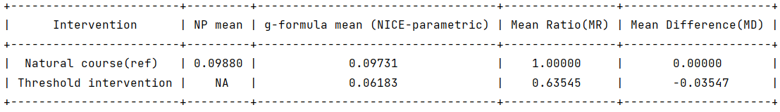
For binary end of follow-up outcomes, the package will output estimates of contrasts in the outcome probability under different user-specified treatment strategies.

Sample syntax:

outcome_name = 'Y'
ymodel = 'Y ~ L1 + A + lag1_A + lag1_L1 + L3 + t0'
outcome_type = 'binary_eof'

g = ParametricGformula(..., outcome_name = outcome_name, outcome_type = outcome_type, ymodel = ymodel, ...)

Running example [code]:

import numpy as np
from pygformula import ParametricGformula
from pygformula.interventions import threshold
from pygformula.data import load_binary_eof

obs_data = load_binary_eof()
time_name = 't0'
id = 'id'

covnames = ['L1', 'L2', 'A']
covtypes = ['binary', 'zero-inflated normal', 'normal']
covmodels = ['L1 ~ lag1_A + lag2_A + lag_cumavg1_L1 + L3 + t0',
             'L2 ~ lag1_A + L1 + lag_cumavg1_L1 + lag_cumavg1_L2 + L3 + t0',
             'A ~ lag1_A + L1 + L2 + lag_cumavg1_L1 + lag_cumavg1_L2 + L3 + t0']

basecovs = ['L3']

outcome_name = 'Y'
ymodel = 'Y ~ L1 + A + lag1_A + lag1_L1 + L3 + t0'
outcome_type = 'binary_eof'

int_descript = ['Threshold intervention']

g = ParametricGformula(obs_data = obs_data, id = id, time_name=time_name,
    int_descript = int_descript,
    Intervention1_A = [threshold, [0.5, float('inf')]],
    covnames=covnames, covtypes=covtypes,
    covmodels=covmodels, basecovs=basecovs,
    outcome_name=outcome_name, ymodel=ymodel, outcome_type=outcome_type)
g.fit()

Output:

Continuous end of follow-up outcome

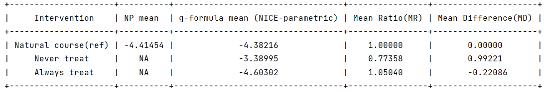
For continuous end of follow-up outcomes, the package will output estimates of contrasts in the outcome mean under different user-specified treatment strategies.

Sample syntax:

outcome_name = 'Y'
ymodel = 'Y ~ C(L1) + L2 + A'
outcome_type = 'continuous_eof'

g = ParametricGformula(..., outcome_name = outcome_name, outcome_type = outcome_type, ymodel = ymodel, ...)

Running example [code]:

import numpy as np
from pygformula import ParametricGformula
from pygformula.interventions import static
from pygformula.data import load_continuous_eof

obs_data = load_continuous_eof()
time_name = 't0'
id = 'id'

covnames = ['L1', 'L2', 'A']
covtypes = ['categorical', 'normal', 'binary']
covmodels = ['L1 ~ C(lag1_L1) + lag1_L2 + t0',
             'L2 ~ lag1_L2 + C(lag1_L1) + lag1_A + t0',
              'A ~ C(L1) + L2 + t0']

basecovs = ['L3']

outcome_name = 'Y'
outcome_model = 'Y ~ C(L1) + L2 + A'
outcome_type = 'continuous_eof'

time_points = np.max(np.unique(obs_data[time_name])) + 1
int_descript = ['Never treat', 'Always treat']

g = ParametricGformula(obs_data = obs_data, id = id, time_name=time_name,
    int_descript=int_descript,
    Intervention1_A = [static, np.zeros(time_points)],
    Intervention2_A = [static, np.ones(time_points)],
    covnames=covnames, covtypes=covtypes,
    covmodels=covmodels, basecovs=basecovs,
    outcome_name=outcome_name, ymodel=ymodel, outcome_type=outcome_type)
g.fit()

Output:

Custom model

The custom fit function needs to contain the input parameters:

ymodel: model statement of the outcome
fit_data: data used to fit the outcome model

and return a fitted model which is used to make prediction in the simulation step.

An example using random forest to fit a outcome model:

def ymodel_fit_custom(ymodel, fit_data):
    y_name, x_name = re.split('~', ymodel.replace(' ', ''))
    x_name = re.split('\+', x_name.replace(' ', ''))
    # get feature and target data to fit ymodel
    y = fit_data[y_name].to_numpy()
    X = fit_data[x_name].to_numpy()
    fit_rf = RandomForestRegressor()
    fit_rf.fit(X, y)
    return fit_rf

The custom predict function needs to contain the input parameters:

ymodel: model statement of the outcome
new_df: simulated data at time t.
fit: fitted model of the custom function

and return a list of predicted values at time t. For survival and binary end-of-follow-up outcomes, the predict function should return the estimated probability. For continuous end-of-follow-up outcomes, it should return the estimated mean.

The example of custom predict function using the random forest model:

def ymodel_predict_custom(ymodel, new_df, fit):
    y_name, x_name = re.split('~', ymodel.replace(' ', ''))
    x_name = re.split('\+', x_name.replace(' ', ''))
    # get feature data to predict
    X = new_df[x_name].to_numpy()
    prediction = fit.predict(X)
    return prediction

Running example [code]:

import numpy as np
import pygformula
from pygformula import ParametricGformula
from pygformula.interventions import static
from pygformula.data import load_continuous_eof

obs_data = load_continuous_eof()

time_name = 't0'
id = 'id'

covnames = ['L1', 'L2', 'A']
covtypes = ['categorical', 'normal', 'binary']
covmodels = ['L1 ~ C(lag1_L1) + lag1_L2 + t0',
             'L2 ~ lag1_L2 + C(lag1_L1) + lag1_A + t0',
              'A ~ C(L1) + L2 + t0']

basecovs = ['L3']

outcome_name = 'Y'

ymodel = 'Y ~ lag1_L2 + L2 + lag1_A + A'

# define interventions
time_points = np.max(np.unique(obs_data[time_name])) + 1
int_descript = ['Never treat', 'Always treat']


def ymodel_fit_custom(ymodel, fit_data):
    y_name, x_name = re.split('~', ymodel.replace(' ', ''))
    x_name = re.split('\+', x_name.replace(' ', ''))
    # get feature and target data to fit ymodel
    y = fit_data[y_name].to_numpy()
    X = fit_data[x_name].to_numpy()
    fit_rf = RandomForestRegressor()
    fit_rf.fit(X, y)
    return fit_rf

def ymodel_predict_custom(ymodel, new_df, fit):
    y_name, x_name = re.split('~', ymodel.replace(' ', ''))
    x_name = re.split('\+', x_name.replace(' ', ''))
    # get feature data to predict
    X = new_df[x_name].to_numpy()
    prediction = fit.predict(X)
    return prediction


g = ParametricGformula(obs_data = obs_data, id = id, time_name=time_name, time_points = time_points,
             int_descript = int_descript,
             Intervention1_A = [static, np.zeros(time_points)], basecovs=['L3'],
             Intervention2_A = [static, np.ones(time_points)],
             covnames=covnames,  covtypes=covtypes, covmodels=covmodels,
             ymodel_fit_custom = ymodel_fit_custom, ymodel_predict_custom=ymodel_predict_custom,
             outcome_name=outcome_name, ymodel=ymodel, outcome_type='continuous_eof')
g.fit()

Note

Note that when there are categorical covariates in the model statement, adding the ‘‘C( )’’ only applies to the default model fitting function. If users want to include it in a custom model fitting function, they need to process the categorical data in addition.